Tutorial
Pyprocessing uses the same coordinate system of Processing, which means that the y axis is directed down. If desired, the user can invert the axis by following these steps:
First, go to the "pyprocessing" folder under the main folder of the library. Then open the file "config.py" and find the code
coordInversionHack = True
which is located at line 22. All you have to do is replace "True" for "False", making the line of code be
coordInversionHack = False
As usual, the x axis has a left to right direction. This means that the coordinate (0,0) is located at the top left corner of the screen. While the user can chose how the y axis is directed, this tutorial will show how the examples are shown without the inversion.
Now we are ready to run our first example and understand how it works. First, create a file and rename it "helloworld.py", then open it with a text editor and insert the following code:
from pyprocessing import *
size(200,200)
line(50,100,150,100)
run()

All you have to do is run it (either with "python helloworld.py" in Linux systems, or by double-clicking in Windows). Now let's understand what each line of code does:
from pyprocessing import*
This simply loads the pyprocessing library into your python file. This line of code is completely necessary in every pyprocessing application you make, since without it Python won't be able to find the pyprocessing functions.
size(200,200)
This sets the size of the your application window. The first number is the horizontal window size, and the second one is its vertical size. Both measures are in pixels.
line(50,100,150,100)
The function line() receives 4 parameters and draws a line in your window. The first two ones represent the coordinate of the start of your line, while the latter two represent the end of your line. So a line connecting the points (50,100) and (150,100) will be drawn.
run()
This piece of code is also always necessary, like
from pyprocessing import *
Due to how pyprocessing is structured, this function call is needed to start the application and actually run all the pieces of code you've written so far. While the import must be placed at the start of your code, the run call must be the last line of your application.
Pyprocessing has many other 2D primitives (geometric shapes), which will be covered in this section.
The point() function is the most basic of them all, and only receives two numbers (representing a coordinate) and draws a point. Now on with geometric shapes:
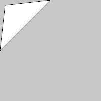
First, we have the triangle() function, which receives 6 numbers (equivalent to 3 coordinates) and draws a triangle. For example,
triangle(10,10,100,0,0,100)
will draw a triangle with the vertices (10,10), (100,0) and (0,100).
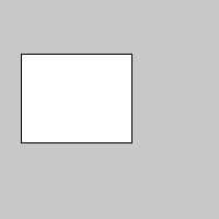
We also have rect(), which receives 4 numbers (the first two represent a point location, and the latter two the horizontal and vertical size of the square), and draws a square. The point represents the location of the upper left corner, meaning that the square is drawn from left to right and up to down, starting at the location defined by the first two numbers. For example,
rect(20,50,100,80)
will draw a square ranging from pixels 20 to 120 in the x axis, and from pixels 50 to 130 in the y axis.
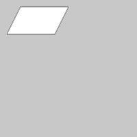
The quad() receives 8 numbers which represent 4 coordinates, and then draws a quadrilateral with the 4 vertices at those coordinates. As example we have
quad(30,10,100,10,80,50,10,50)
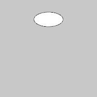
Most circular shapes can be drawn with the ellipse() function. It receives 4 numbers, where the first two indicate the location of the ellipse (a coordinate representing its center) and the latter two its horizontal and vertical sizes. An ellipse with equal horizontal and vertical sizes is actually a circle. We have for example
ellipse(100,40,60,30)
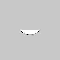
Finally, we have arc(), which is used to draw parts of ellipses (or circles). Its usage is similar to ellipse(), but it receives two angles which represent the start and the end of the arc. Here, the angle 0 represents a vector pointing down, while PI/2 represents a vector pointing to the right, and finally PI represents a vector pointing up.
arc(100,100,60,30,0,PI)
Don't panic if you couldn't understand arc() right now: it'll be covered in other sections and examples.
Pyprocessing also gives you two attributes that can help you drawing your primitives. They are "width" and "height", and they are equal to the horizontal and vertical size of the window, respectively. So if you call
line(20,50,width,50)
you'll always draw a line starting at (20,50) headed all the way to the right end of the window.

In pyprocessing, we represent colors with the ARGB system, which will be explained briefly in this section.
The ARGB system is a way to represent colors with 4 numbers called "color channels". These four channels are called alpha, red, green and blue and each of them represent an individual propriety of a color, and when together they can fully represent any drawable color. The red, green and blue channels indicate "how much" of these colors the original color has. Each channel is represented by an integer number ranging from 0 to 255.
For example, since a pure red color has no blue or green in it, it can be represented by a full red channel and zero green and blue channels, or more specifically R,G,B = 255,0,0. The same works for pure green and blue colors.
Now, we represent all "non-pure" colors by indicating how much red, blue and green they have. For example, we know that by mixing red and green we have yellow, so the yellow color can be represented by R,G,B = 255,255,0. Its also important to remember that for black we have R,G,B = 0,0,0 and for white, R,G,B = 255,255,255.
All colors that have equal R, G and B channels are "grey" colors and can be represented by only one number. For example, the color represented only by the number 100 actually has R,G,B = 100,100,100 and is a tone of grey. Intuitively, the color 0 indicates black while 255 indicates white (both are "grey" colors).

Remember that there is absolutely no need to remember the RGB values for a lot of colors: there are plenty of charts avaliable on the internet that have a fairly big list of colors and their corresponding RGB values.
Finally, we have the alpha channel (or simply A), which doesn't represent a color, but its transparency. A color with A = 0 will be completely transparent, so instead of seeing the color itself, you'll see whats behind it. On the other hand, a color with A = 255 will have no transparency at all, covering the color behind it completely. In other cases (from 1 to 254), you'll see a mix between the color itself and whats behind it. There is no need to fully understand the alpha channel now since we'll see it in other sections. Just remember that if you define a color with only 3 numbers (representing the RGB channels), then pyprocessing will assume that the color has no transparency at all (A = 0).
Now we'll see how to use this knowledge on pyprocessing. This is mainly achieved by the usage of the functions background(), fill() and stroke().
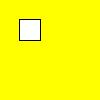
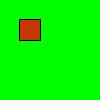
First, the background() function defines the color of the background of your window. In most cases you'll want to call it before drawing anything, since what it really does is draw a square covering your whole window (and this can cover everything you have drawed before). Let's see a basic example where the background color is set as yellow and then a rect is drawn.
from pyprocessing import *
background(255,255,0) #yellow color
rect(20,20,20,20) #rect at location (20,20), width 20 and height 20
run()
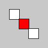
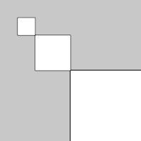
The second function covered in this section is used to indicate the color of a geometric shape that you want to draw. This function is called fill() and its usage is very similar to background(), as it only receives a color. It is important to remember that if you call fill() indicating that you want your geometric shapes to be, for example, purple, then all your future drawings will be purple until you call fill() again. If you only want to draw one red shape and all others to be white, then you need to call fill(255,0,0) before drawing the shape and fill(255) after it. Here's an example that shows this:
from pyprocessing import *
rect(20,20,20,20)
fill(255,0,0) #red color
rect(40,40,20,20)
fill(255) #white (255,255,255)
rect(60,60,20,20)
run()
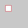
Lastly, we have the stroke() function, which works exactly as fill(), but instead of changing the color of the interior of the shape, it changes the color of its border. Check this simple example to fully understand how it works:
from pyprocessing import *
stroke(255,0,0) #red color
rect(20,20,20,20)
run()
Let's then see an example of the alpha channel in use. Here we'll use the color (255,0,0,200), which is a bit transparent pure red color, to draw a square after setting the background to pure non-transparent green, or (0,255,0). The result is that the red is mixed a little with the green color, just like if you got a semi-transparent red paper and looked to a green wall throught it.
from pyprocessing import *
background(0,255,0)
fill(255,0,0,200) #transparent red
rect(20,20,20,20)
run()
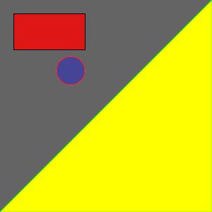
To end this section, let's see an example that uses all the three new functions and several forms of representing a color.
from pyprocessing import *
size(300,300)
background(100)
fill(255,0,0,200) #transparent red
rect(20,20,100,50)
fill(255,255,0) #yellow
stroke(0,255,0) #green
triangle(0,height,width,height,width,0)
fill(0,0,255,80) #transparent blue
stroke(255,0,0) #red
ellipse(100,100,40,40)
run()
In this short section we'll introduce three new simple functions, called strokeCap(), strokeJoin() and strokeWeight(). With them, you can add a pretty cool effect to your geometric shapes, and on the top of that, they're very easy to understand and use.
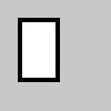
First, strokeWeight() is used to set the thickness of your lines. This includes not only the lines drawn with the line() function, but also the borders of all your geometric shapes. The default is 1 and 8 can be considered a decently thick line.
from pyprocessing import *
strokeWeight(4)
rect(20,20,30,50)
run()
The strokeCap() function is used to indicate how you want the start and end of your lines to be drawn, and doesn't affect borders (since they don't have start or end). Instead of receiving a number, they can receive any of the three modes avaliable, which are PROJECT, ROUND and SQUARE (where SQUARE is the default). In this example you can see how each mode affects the cap of a line.
from pyprocessing import *
strokeWeight(6)
strokeCap(ROUND)
line(20,20,80,20)
strokeCap(PROJECT)
line(20,40,80,40)
strokeCap(SQUARE)
line(20,60,80,60)
run()

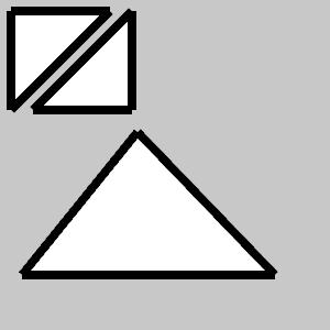
Lastly, the strokeJoin() is used to indicate how you want the joints of the lines that define a shape's border to be drawn. Like strokeCap(), it can receive three modes, which are MITER, BEVEL and ROUND (MITER being the default). Here's an example that shows each mode.
from pyprocessing import *
size(300,300)
strokeWeight(8)
strokeJoin(BEVEL)
triangle(10,10,100,10,10,100)
strokeJoin(MITER)
triangle(120,10,120,100,30,100)
strokeJoin(ROUND)
triangle(20,250,250,250,125,120)
run()
In this section you'll learn how to create continuous applications instead of static ones, giving a lot of power to you new user of pyprocessing. Continuous applications are ones with changing proprieties, for example a triangle that moves around, or an ellipse that gets bigger and then smaller. To use this tool at its full power, you need to learn programming at a reasonable level - and the more you learn, the more you can do with that.
We'll only cover some basic examples since this tutorial doesn't suppose that you are familiar with programming yet. To users more advanced in programming, you'll probably be able to work around and create more complex examples after getting to know how continuous applications work.
Unlike the examples we have seen so far, a continuous application has a different structure. Your application itself will have two functions called setup and draw. The first one is used to start your application, and the second to define how it behaves. The main difference here is that instead of just drawing what you want and stopping, your application will keep doing redraws, making it possible to create things such as moving triangles. The way it does the redraws is to call the draw() function over and over again, while the setup() is only called once, right at the start of your application. The structure of a continuous application is as follows:
from pyprocessing import *
def setup():
   #SETUP SECTION
def draw():
   #DRAW SECTION
run()
In the setup section we'll have calls that are used for setting up attributes and such, and in the draw section we'll have drawing calls.
So let's start with a simple example that is not continuous yet. Suppose we want to draw a thick line on a dark red background. For that, we need 3 calls: strokeWeight, background and line. We'll have the strokeWeight call in the setup area, since it is only setting the thickness of the line (thus a setup call). The line and background calls will be placed in the draw area, since they are actual drawings.
from pyprocessing import *
def setup():
  strokeWeight(6)
def draw():
  background(100,0,0) #dark red
  line(10,10,100,100)
run()

This application doesn't do anything new apparently, right? That's because we don't have anything that changes yet, which will be shown next. Right now, the above example does exactly what the code below does, but the only difference is that it keeps redrawing the dark red background and the line over and over - this obviously can't be noticed since we're drawing the same thing above itself.
from pyprocessing import *
strokeWeight(6)
background(100,0,0)
line(10,10,100,100)
run()
Now let's see an example of a real continuous application in pyprocessing. We'll change the color of the background gradually by changing its value inside the draw block. In this example we'll make the background start having the color (0,0,0) - black, and gradually end up at (255,0,0). At this point, it'll get black and start rising again. For that, we're going to assign a variable "R" to represent the red component of its color, and then make it change. The value assingment will be placed in the setup block, while the background() call will be in the draw block.
from pyprocessing import *
def setup():
  global R
  R = 0
def draw():
  global R
  background(R,0,0)
run()
The "global R" line was necessary because we defined the variable R in the setup section but we also used it in the draw section. Everytime you create a variable in the setup area which will be used in the draw area, you'll have to add a line "global variablename". If you don't really understand why this is necessary, there is no need to worry as understanding this mechanism isn't necessary for basic pyprocessing users.
Now what our application does so far is, basically, draw a black background. This is because we haven't changed the value of R yet (its value is 0 and doesn't change). Let's make it gradually go to 255 and then back to 0, continously. To do that, let's use this:
if R == 255: R = 0
else: R = R + 1
What this piece of code does is basically check if the value of R is 255 - if it is, then we reset its value to 0, if not, we increase it by 1. Now we only need to add that to the draw section.
from pyprocessing import *
def setup():
  global R
  R = 0
def draw():
  global R
  if R == 255: R = 0
  else: R = R + 1
  background(R,0,0)
run()
Now we can follow this schema to create many different continuous applications. Instead of changing a color value, let's change a triangle's position.
from pyprocessing import *
def setup():
  size(200,200)
  global vx
  vx = 0
def draw():
  global vx
  background(200)
  if vx == 100: vx = 0
  else: vx = vx + 1
  triangle(vx,0,0,100,200-vx,100)
run()
And now let's change the position of a circle's center. Here we'll make the circle orbit around the center of the window (with an orbit of radius 50) by making its center be at "width/2 + 50*sin(x),height/2 + 50*cos(x)" and then change the angle x.
from pyprocessing import *
def setup():
  global x
  size(200,200)
  x = 0
def draw():
  global x
  background(200)
  x = x + 0.1
  ellipse(width/2 + 50*sin(x), height/2 + 50*cos(x), 10, 10)
run()
Finally, let's make a triangle rotate by making each of its vertices orbit, just like the circle of the previous example. The vertices need to be one third of a circle ahead of eachother, so the first one will use the angle "x", the second "x + 2*PI/3" and the third "x + 4*PI/3" - just remember that a full circle equals 2*PI.
from pyprocessing import *
def setup():
  global x
  size(200,200)
  x = 0
def draw():
  global x
  background(200)
  x = x + 0.1
  triangle(width/2 + 50*sin(x), height/2 + 50*cos(x), width/2 + 50*sin(x
 + 2*PI/3), height/2 + 50*cos(x + 2*PI/3), width/2 + 50*sin(x + 4*PI/3),
 height/2 + 50*cos(x + 4*PI/3))
run()
There's no need to worry if you feel unsafe when working with such mathematical formulae. Later on we'll see some functions that can make your life easier and make you not worry about equations to draw things. Before heading to the next section, please try to create some continuous applications by yourself until you're safe with reading draw() sections and knowing how the drawing will progress.
This is another powerful section, and here you'll learn how to make the user interact with your continuous application by using the mouse and the keyboard.
Let's start with the simplest of them, which is the keyboard.
If we want our application to interact with a user's keyboard, we have to create another function called keyPressed() that pyprocessing will call everytime a key is pressed. Our application will now look like this:
import pyprocessing
def setup():
  #SETUP SECTION
def draw():
  #DRAW SECTION
def keyPressed():
  #KEYBOARD SECTION
run()
Inside this section, we can use some preset variables (similar to width and height) which give us information about the state of the keyboard. The first variable is called "key.char" and its value will be the character that was pressed. Here's a quick example to show how it works:
from pyprocessing import *
def setup():
  global col
  col = 0
def draw():
  global col
  background(col)
def keyPressed():
  global col
  if key.char == "c": col = 200
run()
Simply, when the user press the key "c", the variable col will have its value set to 200, and the background will turn grey.
The second variable is called "key.code" and returns the code of the pressed key. This is useful if you want to check for keys like backspace, enter or directional arrows. Here's a list of some important key codes and an example:
Space: 32 Ctrl: 65507 Backspace: 65288 Up: 65362 Left: 65361 Down: 65364 Right: 65363
from pyprocessing import *
def setup():
  global vx, vy
  size(200,200)
  vx = width/2
  vy = height/2
def draw():
  global vx,vy
  background(200)
  ellipse(vx,vy,10,10) #circle at location (vx,vy) and radius 10
def keyPressed():
  global vx,vy
  if key.code == 65362: vy = vy - 5 #decrases vy if the key was up arrow
  if key.code == 65361: vx = vx - 5 #decrases vx if the key was left
arrow
  if key.code == 65364: vy = vy + 5 #increases vy if the key was down
arrow
  if key.code == 65363: vx = vx + 5 #increases vx if the key was right
arrow
run()
Now, mouse interaction. The mouse can have 4 functions and has some preset variables as well. The functions are:
mouseClicked() - called when a mouse button is pressed and released mouseDragged() - called when the mouse is moved while a button is pressed mouseMoved() - called when the mouse is moved without buttons pressed mousePressed() - called when a mouse button is pressed
So basically, we can have applications with a structure like:
import pyprocessing
def setup():
  #SETUP SECTION
def draw():
  #DRAW SECTION
def keyPressed():
  #KEYBOARD SECTION
def mouseClicked():
  #MOUSE CLICKED SECTION
def mouseDragged():
  #MOUSE DRAGGED SECTION
def mouseMoved():
  #MOUSE MOVED SECTION
def mousePressed():
  #MOUSE PRESSED SECTION
run()
But remember that you don't need to make all those functions. Usually only one or two will be enough if you want mouse interaction. The preset variables that you'll use are "mouse.x" and "mouse.y", which indicate the x and y components of the mouse's current coordinate.
Here's an example that only uses mouse.x and mouse.y:
from pyprocessing import *
def setup():
  size(200,200)
def draw():
  background(200)
  ellipse(mouse.x,mouse.y,10,10) #draws a circle at the location of the
mouse and radius 10
run()
We didn't need to create any of the mouse interaction functions because we don't need to do anything when the mouse is clicked, dragged or moved - we only draw a circle at its current position, and that's it.
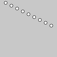
And finally an example using mouseDragged():
from pyprocessing import *
def setup():
  global coords
  coords = []
  size(200,200)
def draw():
  global coords
  background(200)
  for i,j in coords: point(i,j)
def mouseDragged():
  global coords
  coords.append((mouse.x,mouse.y))
run()
In this example we start by creating an empty list
coords = []
which will store the coordinates of the points that will be drawn. When the user drags his mouse, the current position of the mouse is added to the coords list:
coords.append((mouse.x,mouse.y))
Finally, we draw one point for each coordinate in the coords list:
for i,j in coords: point(i,j)
This section is dedicated to images in general. Images are simply a big amount of color values, each representing one pixel. A 800x600 image, for example, has 800 pixels in width and 600 in height, thus a grand total of 480000 pixels. Each pixel is nothing more than a color value - ARGB.
The first function that we need to know is loadImage(), which needs you to give the location of an image in your computer and then loads it into a variable of your choise. The usage is as follows:
f = loadImage("C:/Pictures/picture01.jpg")
After that, you'll be able to work with the image you just loaded by using the variable "f" (in this example). We'll use "f" to indicate the variable you chose to load your image into, but remember that it could have been anything else. An image has two very important attributes that represent its width and height - in this example, they can be accessed by f.width and f.height.
To display an image, the function you'll need is "image()", which needs 3 arguments: an image and the two values of a coordinate - in this case, the coordinate will represent the location of the upper left point of the image. Try running this example (with an image of your choice):
from pyprocessing import *
f = loadImage("LOCATION OF THE IMAGE GOES HERE")
size(f.width,f.height)
image(f,0,0)
run()
We used
size(f.width,f.height)
to make our application window have the same size of the image, so it doesn't get cropped or anything like that.
Now we have two ways of manipulating our image. The first one is to apply an image filter, which is actually a premade effect. We can apply a filter with the call
f.filter()
and one argument - the filter name. Currently, pyprocessing has the following filters implemented:
GRAY: Makes the image black and white. INVERT: Invert the colors of an image. BLUR: Applies a blur effect to the image according to the second parameter. OPAQUE: Makes the image completely opaque (Alpha = 255) THRESHOLD: Receives a second argument between 0 and 1 that will be used as threshold to every pixel - the ones that are below it turn black and the ones above turn white. The argument represents a color between black (0) and white (1). POSTERIZE: Limits each color channel to "n" channels, where "n" is a second argument needed for this filter. ERODE: Reduces light. DILATE: Increases light.
Here are some examples using the image filters:
from pyprocessing import *
f = loadImage("LOCATION OF THE IMAGE GOES HERE")
size(f.width,f.height)
f.filter(GRAY)
image(f,0,0)
run()
from pyprocessing import *
f = loadImage("LOCATION OF THE IMAGE GOES HERE")
size(f.width,f.height)
f.filter(THRESHOLD,0.7)
image(f,0,0)
run()
from pyprocessing import *
f = loadImage("LOCATION OF THE IMAGE GOES HERE")
size(f.width,f.height)
f.filter(POSTERIZE,5)
image(f,0,0)
run()
Now the second way to manipulate an image is to work directly with its pixels by using the functions "get()" and "set()". The "get()" function needs two arguments that indicate a coordinate and returns the pixel of the image at that location, while "set()" needs a color and a coordinate and sets the pixel at that coordinate with the indicated color. Remember that both functions work with the ARGB value of a color, so "get()" will return an ARGB value and "set()" requires an ARGB value. You can use the "color()" function to convert your 3 or 4-value colors to ARGB, like:
color(200,0,100)
And you can get separate channels off an ARGB value by using the functions "alpha()", "red()", "blue()" and "green()". For example, red(color(200,0,100)) equals 200.
Now let's make an example that runs through all the pixels of an image and changes its red channel by its green channel. First, to get the the
of a pixel, at the coordinate (50,50), we'll need:
col = f.get(50,50)
R = red(col)
G = green(col)
B = blue(col)
And then we need to compose the new ARGB value, which will have the red and green channels traded:
newcol = color(G,R,B)
And finally make the pixel(50,50) have the new color:
set(50,50,newcol)
In the end, we have:
from pyprocessing import *
f = loadImage("LOCATION OF THE IMAGE GOES HERE")
size(f.width,f.height)
for i in range(f.width):
  for j in range(f.height):
    col = f.get(i,j)
    R = red(col)
    G = green(col)
    B = blue(col)
    newcol = color(G,R,B)
    f.set(i,j,newcol)
image(f,0,0)
run()
Don't try to run this example with large images because this is a very slow way to do what we're doing - later on we'll find more performance-friendly ways of manipulating an image's pixels.
The transform functions are powerful tools to help you make your application without having to do much math, and give you more control regarding the coordinates of your window. In this section we're going to learn how to use scale(), translate() and rotate(), altough there are other powerful functions that are going to be covered later in other sections.
First, scale() is used as a multiplier to the arguments you use to draw geometric shapes. It receives one or two numbers and set them as multipliers to the x and y parameters of all your future shapes. For example, a x factor of 2 will make your rects have doubled width - and also be drawn at double the distance specified. If you only give scale() one number, it sets it as the multiplier for both x and y.
For example, if we set the x and y multipliers to 2 by using scale(2), then when we call rect(10,10,20,20) then the rect will be drawn at location (20,20) and will have width and height of 40.
One very important propriety of all transform functions is that they are cumulative, meaning that if you call scale(2) twice, then you'll actually have a multiplier of 4. The factor is reset to 1 each time draw() is ran, meaning that if you have a scale() call inside your draw section, then it won't change the factor cumulatively at each redraw.
Here's one example showing a basic static use of scale():
from pyprocessing import *
size(200,200)
rect(100,100,100,100) #draws a rect at (100,100) with width and height
100
scale(0.5) #sets the scale factor to 0.5
rect(100,100,100,100) #draws a rect at (50,50) with width and height 50
scale(0.5) #sets the scale factor to 0.25
rect(100,100,100,100) #draws a rect at (25,25) with width and height 25
run()
And now a continuous example:
from pyprocessing import *
def setup():
  global factor
  factor = 1
  size(200,200)
def draw():
  global factor
  scale(factor)
  rect(100,100,100,100)
  factor = factor/2.0
run()

Here we're first setting factor as 1, and at each redraw it'll be divided by 2. That makes our rect to be drawn at half its position, width and height during each draw call. Since we don't have a background() call inside our draw section, we can see the rects that have been drawed in previous frames.
The second transform function is translate(), and it receives two parameters that indicate the x and y translation for your axis, respectivelly. Having a translation means that your your x and y axis are now in a new position of your screen. Remember that the default location for them was the upper left corner of your window? With translate() you can move your axis to whereever you want.
If, for example, we call translate(20,10), then the location of our (0,0) point will now be the location that the point (20,10) used to have. Let's see an example showing that:
from pyprocessing import *
translate(20,10)
ellipse(0,0,10,10) #draws a circle at (20,10) with radius 10
run()

Just like scale(), the transform function is cumulative, meaning that two transform(10,20) calls will have our (0,0) coordinate placed at our old (20,40) location.
Let's see a continuous example that uses transform():
from pyprocessing import *
def setup():
  size(200,200)
def draw():
  for i in range(9):
    translate(20,10)
    ellipse(0,0,10,10)
run()
We're just calling translate(20,10) followed by ellipse(0,0,10,10) 9 times. This is equivalent to calling ellipse(20,10,10,10), then ellipse(40,20,10,10), then ellipse(60,30,10,10) and so on. Quite simple, right?
Lastly, the rotate() function rotates our x and y axis around an angle that is received as a parameter. This is probably the most useful transform since it is an alternative to math involving sin and cos operations.
from pyprocessing import *
size(200,200)
rect(100,0,50,50)
rotate(PI/4.0)
rect(100,0,50,50)
run()
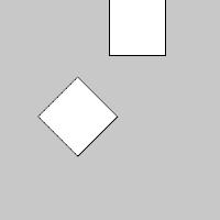
With rotate(PI/4.0), we defined a rotation factor of 45 degrees. The coordinate (100,0) that indicates the upper left vertex of the rectangle was rotated by 45 degrees together with the rect itself.
Let's see an example that uses both translate() and rotate() to draw triangles:
from pyprocessing import *
size(200,200)
translate(width/2,height/2)
for i in range(10):
  rotate(2*PI/10)
  triangle(0,-100,50,50,-50,50)
run()
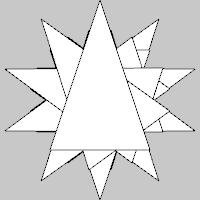
First we're setting our (0,0) coordinate to the middle of our screen with:
translate(width/2,height/2)
Then we're calling rotate(2*PI/10) followed by triangle(0,-100,50,50,-50,50) 10 times. First we're drawing a triangle in the middle of the screen and then we're having rotations of 36 degrees all the way to a full 360 degrees rotation.
To end this section, let's see two examples that use some tools that we've already learned in the previous sections.
from pyprocessing import *
size(200,200)
translate(100,100)
stroke(40,70,0,90)
fill(100,0,0,90)
for i in range(10):
  rotate(2*PI/10)
  triangle(0,-100,50,50,-50,50)
run()
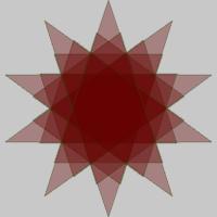
This one is just like the previous example, but uses transparent fill and stroke colors for a cool effect.
from pyprocessing import *
def setup():
  global offset
  offset = 0
  size(200,200)
  stroke(40,70,0,90)
def draw():
  global offset
  translate(100,100)
  fill(100,0,0,10)
  rotate(offset)
  for i in range(10):
    rotate(2*PI/10)
    triangle(0,-100,50,50,-50,50)
  fill(100,100,0,90)
  rotate(-2*offset)
  for i in range(20):
    rotate(-PI/10.0)
    rect(-20,-20,10,40)
  fill(29,84,201,6)
  for i in range(10):
    scale(0.8)
    ellipse(0,0,200,200)
  offset += PI/70
run()
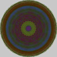
Now this one is kind of more complex. Basically you draw a triangle with a different rotation each frame in order to make the spiral dark red saw. Then you draw yellow rectangles (again, each frame with a different rotation angle) in the middle in order to make the smaller saw. And finally a blue circle to make the purple degradé due to the alpha channel mix.